Enrichment Analysis

Enrichment analysis…

Note: Will include content from the research paper, once it becomes available

Functional Enrichment Analysis (FEA)

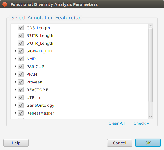
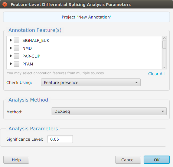
Functional enrichment analysis… You may specify what expression data type to use – genes, proteins, or transcripts – for the analysis, and the corresponding test and background lists to use. Available application lists are provided but you may use any previously generated list file. You also need to specify what annotation features to test for and some analysis package required parameters.

Note: Will include content from the research paper, once it becomes available

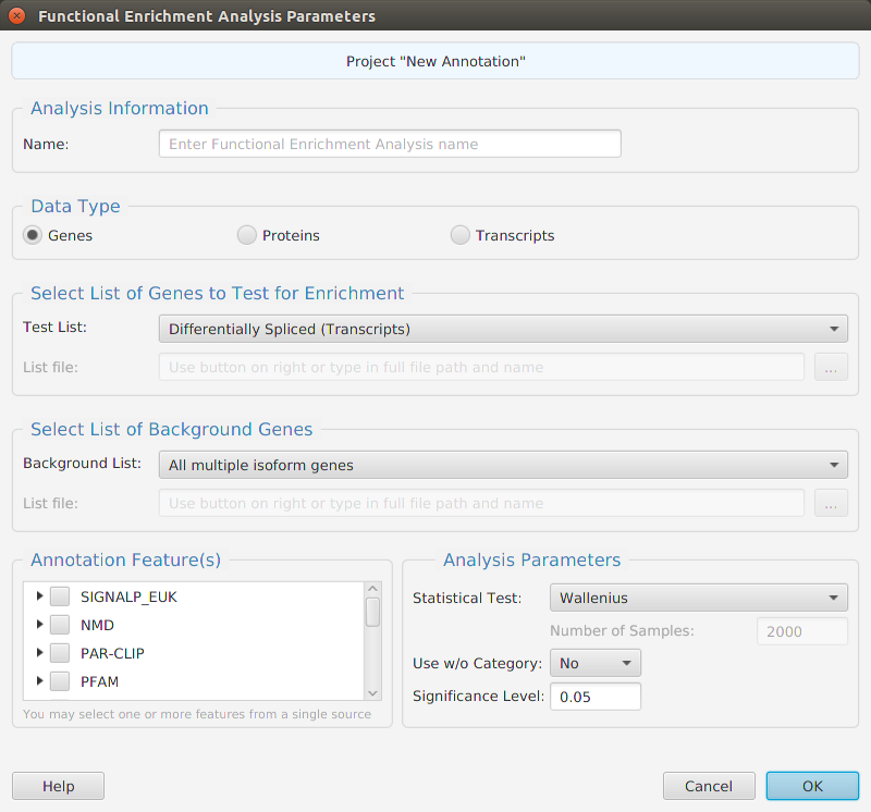
When using the application, all FEA parameters are described in the Help page which can be accessed via the Help button located on the bottom left of the dialog window.

goseq

Goseq provides “…”.You may view the documentation and installation instructions at:
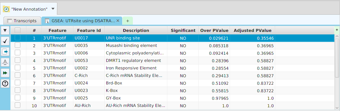
 

FEA Results

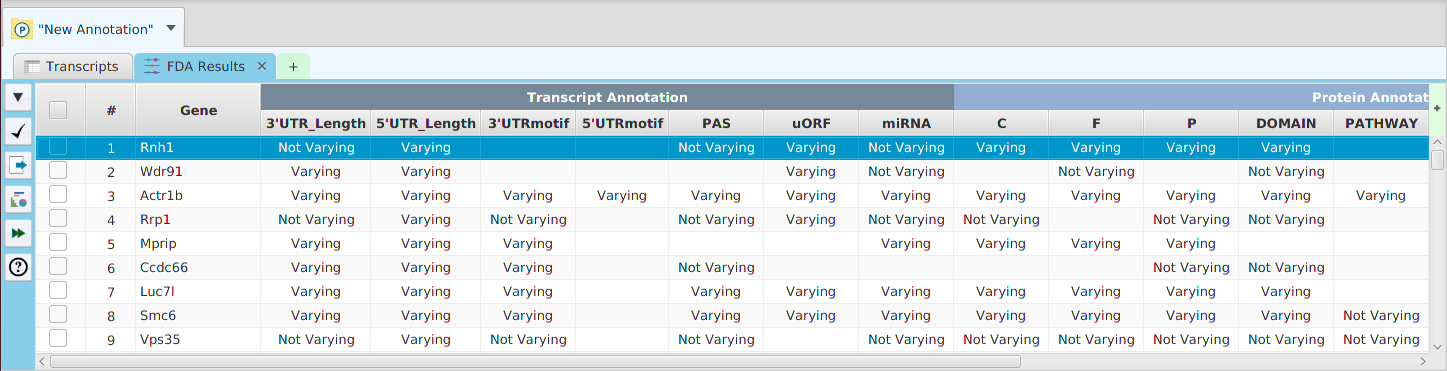
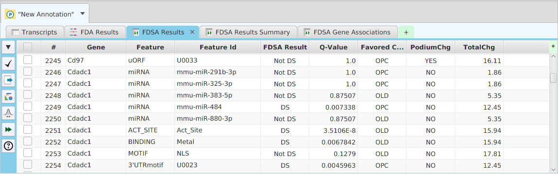
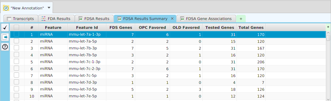
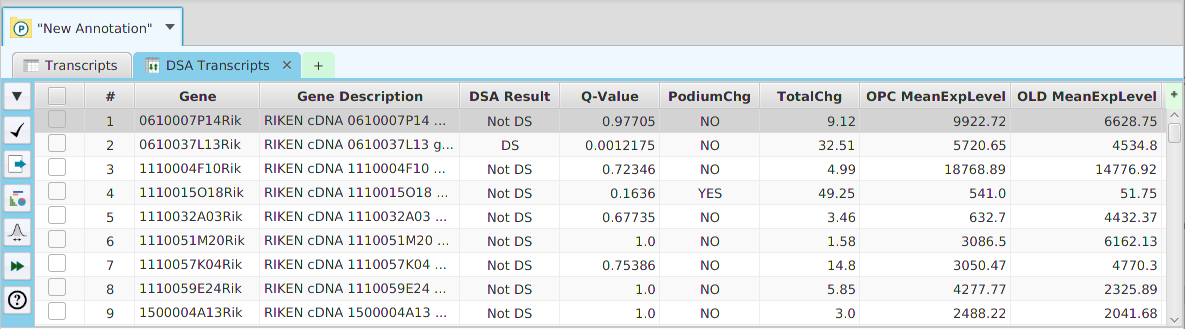
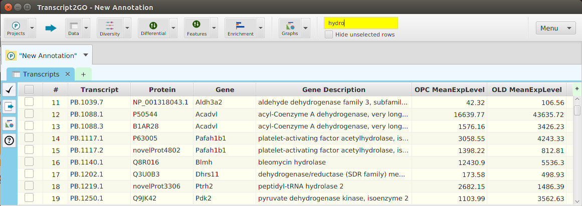
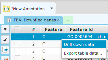
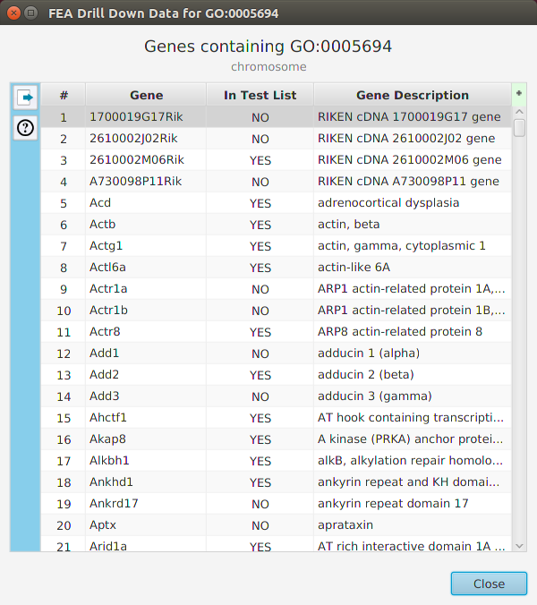
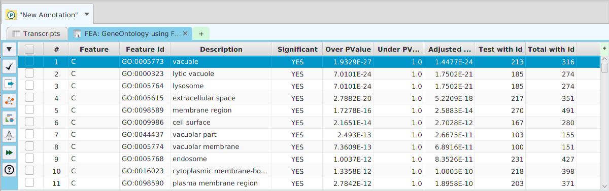
The FEA results are displayed in a table on the FEA Results subtab. The subtab is contained in the project data tab located in the top tab panel, see image below. Each table row displays the results, Significant – Yes/No, for a given annotation feature as well as over/under and adjusted P-Values. The number of test genes and total genes containing the feature are also shown.

Enriched Features Cluster Analysis

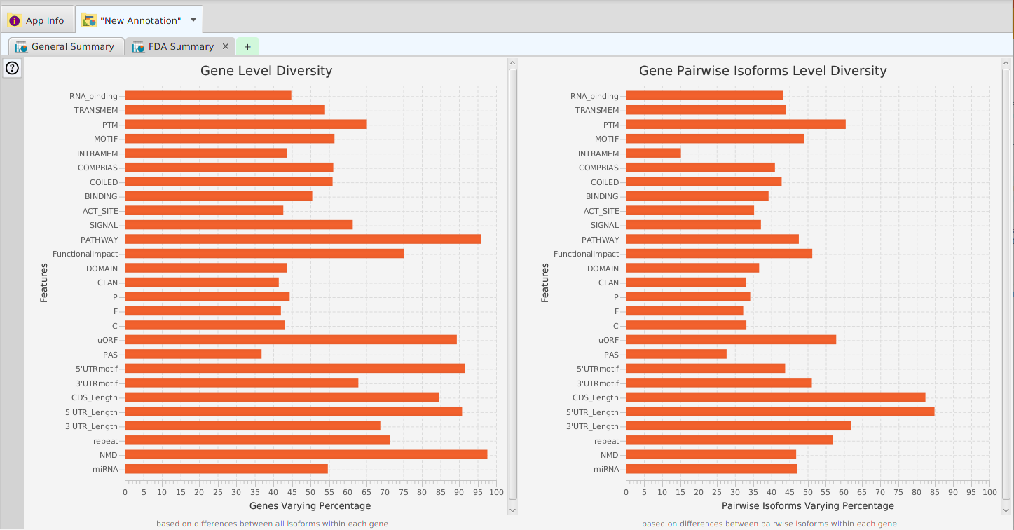
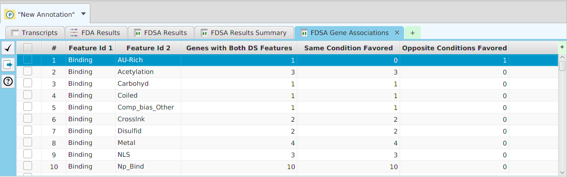
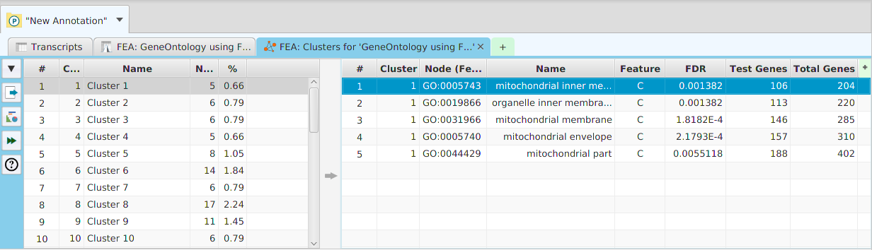
The option to run Cluster Analysis on the enriched features from the FEA results is provided. The cluster analysis results can be seen below. The table on the left displays the clusters while the table on the right displays the nodes for the selected cluster(s). You may select multiple clusters to see their combined nodes.

Gene Set Enrichment Analysis (GSEA)

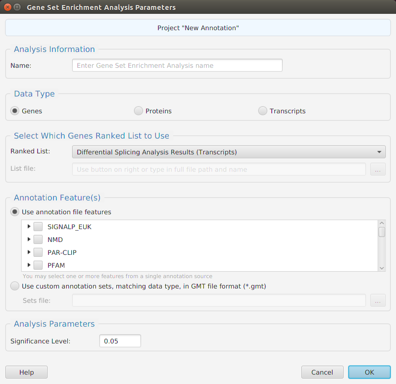
Gene set enrichment analysis… You may specify what expression data type to use – genes, proteins, or transcripts – for the analysis, and the corresponding ranked list to use. Available application ranked lists are provided but you may use any previously generated ranked list file. You also need to specify what annotation features to test for either by selecting from list or providing your own annotation sets in GMT file format.

Note: Will include content from the research paper, once it becomes available

When using the application, all GSEA parameters are described in the Help page which can be accessed via the Help button located on the bottom left of the dialog window.

GOglm

GOglm provides “…”.You may view the documentation and installation instructions at:


GSEA Results
The GSEA results are displayed in a table on the GSEA Results subtab. The subtab is contained in the project data tab located in the top tab panel, see image below. Each table row displays the results, Significant – Yes/No, for a given annotation feature as well as over and adjusted P-Values.

Annotation Feature Analysis

The analysis of annotation features provides…

Note: Will include content from the research paper, once it becomes available

Annotation Features Diversity Analysis (FDA)

The diversity of annotation features among gene isoforms…

Note: Will include content from the research paper, once it becomes available

When using the application, all FDA parameters are described in the Help page which can be accessed via the Help button located on the bottom left of the dialog window.

FDA Results
The FDA results are displayed in a table on the FDA Results subtab. The subtab is contained in the project data tab located in the top tab panel, see image below. Each table row displays the diversity results for a given gene. The result columns are grouped into transcript, protein, and genomic annotations. Each column within a group displays the Varying/NotVarying results for the corresponding feature. Blank row cells indicate the feature was not present for the given gene.

FDA Results Summary
The FDA Summary data visualization subtab provides results summary information. The subtab is contained in the project data visualization tab located in the bottom tab panel, see image below. The chart on the left provides varying percentages for each annotation feature at the gene level. The chart on the right provides varying percentages for each annotation feature using pairwise gene isoforms comparisons. As expected, the varying percentages using the pairwise isoforms are lower.

Differential Feature Inclusion Analysis (DFI)

To perform Feature-level differential splicing analysis, you choose what features you will like to include. You also need to specify if you want the features among gene isoforms to be compared using presence or genomic position overlap. The former just checks for the feature being present and having the same count. The latter checks for a genomic position overlap match for each instance of the feature. Just like in regular DIU, you may choose which R package to use, DEXSeq or edgeR.

Note: Will include content from the research paper, once it becomes available

When using the application, all DFI parameters are described in the Help page which can be accessed via the Help button located on the bottom left of the dialog window.

DEXSeq
DEXSeq provides “…”.You may view the documentation and installation instructions at:


edgeR
EdgeR provides “…”.You may view the documentation and installation instructions at:


DFI Results
The DFI results are displayed in a table on the DFI Results subtab. The subtab is contained in the project data tab located in the top tab panel, see image below. Each table row displays the same information as in the regular DFI, the difference being in the rows containing a specific annotation feature in addition to the gene.

DFI Results Summary
The DFI results summary table summarizes the results by feature. For each feature, it displays the number of feature DIU genes detected as well as the number of tested and total genes. Tested genes is the actual number of genes tested for DIU, that is genes having multiple isoforms and varying feature. Total genes is the number of genes containing the feature. The number of DIU genes favoring each condition is also displayed. Each table row displays the same information as in the regular DIU, the difference being in the rows containing a specific annotation feature in addition to the gene.

DFI Results Gene Association
The DFI results gene association table explores the association of two features to any given gene. For each pair of features, it displays the number of genes where both features were found to be DS. In addition, the counts for genes where the features were favored in the same or opposite conditions are shown.

Differential Isoform Usage

Differential splicing analysis can be performed for transcripts or proteins, see image below. Just like in the normal DIU using transcripts, using proteins allows checking for differential splicing at the protein level. Protein levels for DIU are calculated using the sum of their corresponding normalized transcript expression levels within the same gene. You may choose which R package to use, DEXSeqor edgeR, for DIU Analysis.

When using the application, all DIU parameters are described in the Help page which can be accessed via the Help button located on the bottom left of the dialog window. Also, be aware that you do not need to rerun the analysis to change the significance level value: a menu button is provided in the subtab menu bar, see Subtabs Menu Bar section, to change the significance level value and recalculate the DS/NotDS results.

DEXSeq

DEXSeq provides “…”.You may view the documentation and installation instructions at:


edgeR

EdgeR provides “…”.You may view the documentation and installation instructions at:


DIU Results

The DIU results are displayed in a table on the DIU Results subtab. The subtab is contained in the project data tab located in the top tab panel, see image below. It includes basic informational fields such as gene and gene description. It also includes the results, DS/NotDS, Q-Value or P-Value, depending on the R package used, Total Change, and Podium Change. Podium change is used to indicate if the most expressed transcript or protein, depending on the data type selected, changed between conditions. The mean normalized expression levels for each condition are shown for each row.

Be aware that you do not need to rerun the analysis to change the significance level value: a menu button is provided in the subtab menu bar, left part of the image, to change the significance level value and recalculate the DIU/NotDIU results. When running the application, a description of all fields in the result table can be viewed using the subtab Help button.

Differential Expression Analysis

Differential Expression Analysis (DEA) performs statistical testing to determine if a given difference in read counts, between conditions, is significant or just due to random variations. You may run DEA at the gene, protein, and transcript levels, see image below. Protein and gene expression levels are calculated using the sum of their corresponding normalized transcript expression levels. You may also choose which R package to use, NOISeq or edgeR.

When using the application, all DEA parameters are described in the Help page which can be accessed via the Help button located on the bottom left of the dialog window.

NOISeq

NOISeq provides “differential expression between two experimental conditions with no parametric assumptions”.You may view the documentation and installation instructions at:

edgeR

EdgeR provides “differential expression analysis of RNA-seq expression profiles with biological replication. Implements a range of statistical methodology based on the negative binomial distributions, including empirical Bayes estimation, exact tests, generalized linear models and quasi-likelihood tests”.You may view the documentation and installation instructions at:

DEA Results

The DEA results are displayed in a table on the DEA Results subtab. The subtab is contained in the project data tab located in the top tab panel, see image below. It includes basic informational fields about gene, transcripts, or proteins depending on the DEA data type selected. It also includes the DEA test results, DE/NotDE and Up/Down regulation if DE, Probability or P-Value, depending on the R package used, and the Log2 of the fold change (Log2FC). The mean of the normalized expression levels for each condition are shown for each row.

Be aware that you do not need to rerun the analysis to change the significance level value: a menu button is provided in the subtab menu bar, left part of the image, to change the significance level value and recalculate the DE/NotDE results. When running the application, a description of all fields in the result table can be viewed using the subtab Help button.

Ad Hoc Query

All project data and analysis results in the application are displayed in table format. The ability to interactively search and filter the information is an essential part of the application and two complementary functions are provided: a simple search text box and a more powerful row selection query by column filter.

Searching for a specific item in a table is a commonly used function when viewing a data table. The search text box located in the top toolbar of the application provides basic search functionality. As you type, only the table rows containing the entry will be displayed. The search is case insensitive and applies only to id, name, and description fields. Numeric, Yes/No, etc. fields are not searched. It provides a quick and simple way to find specific rows, i.e genes, transcripts, etc. There are some search functionality and behavior you should be aware of:

  • The search is only applicable to data tables for subtabs contained in the Project Data Tab
  • To search a specific table, first select the table by clicking on any row and then select the search text box and type
  • Rows that contain the typed search text will be displayed, all other rows will be hidden
  • Even though there is a single application search text box, the typed search text for each individual subtab table will be displayed when the subtab table is selected
  • Notice how the table background changes to yellow when the data display is being filtered – it is intended to make you aware that the data has been filtered
  • To undo the search filter, just clear the contents of the search text box for the selected subtab table

Row Selection Query

The row selection query feature, provides a more powerful way to filter table data rows. There are multiple ways to select table data rows:

  • Manually by clicking on the corresponding row selection checkbox column, left most table column
  • By clicking on the row selection button on the subtab menu bar and then choosing one of the row selection menu items
  • By right-clicking on a table column and specifying the filtering criteria for that column

If you choose the “Add/Remove row selections…” menu item or right-click on the table column, you will be provided with a criteria editor so that you may specify the filtering criteria. The filtering options available on the editor will change based on the content type of the column being filtered.

There are some row selection functionality and behavior you should be aware of:

  • To only show the selected rows, check the “Hide unselected rows” checkbox located on the top tool bar
  • Notice how the table background changes to yellow when the data display is being filtered – it is intended to make you aware that the data has been filtered
  • To clear the row selection query filtering, use the “Deselect all rows” menu item selection in the subtab menu bar row selection button
  • You may also clear the row selection query filtering by using the table row selection column header checkbox
  • You may also display all rows without clearing the selected rows by unchecking the “Hide unselected rows” checkbox

Export Data and Images

You may export all table data and data visualization images – such as charts, graphs, etc. – in the application to file.

Export Data

The export table data function may be accessed via context-sensitive menu or via the Export menu button on the subtab menu bar. Once invoked, a data export dialog window will be displayed, see below:

The data export dialog provides multiple options for which data to export. The options will vary based on the data table but the most common options are:

  • Table rows – include all data shown for each table row. Note that only visible columns are exported. You may show/hide columns using the table’s + menu
  • Items list (IDs only) – export only the item IDs, where item refer to genes, transcripts, etc.
  • Items ranked list (IDs and values) – export the item IDs and primary statistical result values, where item refer to genes, transcripts, etc.

In addition, options are provided for which table rows to export:

  • Include all data – select to export all table data rows
  • Include only selected rows – select to export ONLY selected table data rows

Once you select the data to export, the standard ‘specify file’ dialog window, provided by the Operating System in your computer, will be displayed so you can choose what file to export the data to.

Export Images

Just like in the data export, the image export function may be accessed via context-sensitive menu or via the Export menu button on the subtab menu bar. However, there are no options for exporting images; once the export function is invoked, the ‘specify file’ dialog window will be opened directly. All images are exported in Portable Network Graphics (PNG) file format.

Data Drill Down

The ability to see the underlying data details can be extremely helpful and is provided, where relevant, via context-sensitive menus. As previously discussed in the Context-Sensitive Menussection, the data table row that you right-click on will determine the contents of the drill down data. For example, in the FEA results for Gene Ontology features window, shown below, the context menu provides a selection to drill down data.

Once selected, the drill down data window will be displayed, see image below. Note the drill down data is for “GO:0005694” which is the selected table row. You may export the drill down table data and, for this specific example, view gene data visualization for specific genes via context menu.

Data Visualization

Data visualization is a powerful tool for recognizing patterns, detecting correlations, and better understanding the data. TAPPAS provides a diverse set of visual elements for this purpose:

  • Summary graphs, charts, and plots
  • Distribution charts
  • Annotation features visualization graphs for gene, proteins, and transcripts
  • Expression level data density and PCA plot
  • Cluster network graphs
  • GO terms directed acyclic graphs
  • Venn diagrams
  • Other miscellaneous visualization displays
Accessing Data Visualizations

Data visualization display subtabs are provided for most data tables in the application. The easiest way to access data visualization for a specific table is to click on the data visualization button provided in the data subtabs and then choose from one of the menu item selections, see image below. Alternatively, you may use the Graphs menu button on the application’s top tool bar and select accordingly.

Once you make a selection, the data visualization subtab will be shown in the project’s data visualization tab, see image below.

Gene Data Visualization

tappAS provides a self contained display tab for gene data visualization. It includes a comprehensive set of data visualization subtabs for gene annotation features down to the individual isoforms. The following subtabs are included:

  • Transcripts – display of transcript annotation features
  • Proteins – display of protein annotation features
  • Genomics – full genomic view showing exons, introns, and genomic annotation features
  • Gene Ontology – display of gene ontology graph for GO annotation features
  • Expression Charts – display of expression level charts for gene, proteins, and transcripts
  • Annotation Features Diversity – cross table display of annotation features and transcripts/proteins
  • Annotation File Data – display of all annotation features for this gene contained in the annotation file

To access the visualization data for a specific gene, right click on the table row containing the gene of interest, for example the gene data table or the DIU results table, and click on the ‘Show gene data visualization’ menu item selection in the context menu. See Context-Sensitive Menus section. You may use the slide control buttons below to see all gene data visualization subtabs snapshots.

Application Interface

tappAS is a Java application and its Graphical User Interface (GUI) is based on JavaFX. Using JavaFX allows the application to work across multiple Operating Systems (OS) and provide the same look and feel of native applications. In addition, JavaFX allows the application to provide the rich set of features expected from a modern GUI application.

GUI Layout

The application layout consists of 3 main sections: a top tool bar and two tab panels, a data tab panel on top and a data visualization tab panel on the bottom, see image below.

Application GUI Layout
A. Top Tool Bar

The top tool bar provides access to all the high level functionality in the application. Starting on the left, it contains multiple menu buttons:

  • Projects – provides access to all the project management functions: create, open, close, list, and delete
  • Data – provides access to all the project data: transcripts, proteins, genes, and original expression matrix. In addition, it provides a menu selection to reinput the project data
  • Diversity – provides access to all the annotation features diversity management functions: run analysis, view and clear analysis results
  • Differential – contains all the differential expression and splicing analysis management functions: run analysis, view and clear analysis results
  • Features – contains all the enrichment analysis, FEA and GSEA, management functions: run analysis, view and clear analysis results

Located after the menu buttons, are the data table search text field and the filter checkbox controls. These controls apply to the currently selected data table, in one of the subtabs below, and as their name implies, are used for searching and table row filtering purposes. Finally, all the way on the left, there is a menu button to access miscellaneous application functions.

B. Top (Data) Tab Panel
The top tab panel is used to display data tabs for all opened projects.
C. Bottom (Data Visualization) Tab Panel
The bottom tab panel is used to display data visualization tabs for all opened projects. In addition, gene data visualization tabs and the global application tab are also displayed here.
D. Data Tab
Data tabs, one per project, contain project data subtabs.
E. Data Visualization Tab
Data visualization tabs, one per project, contain project data visualization subtabs.
F. Gene Data Visualization Tab
Gene data visualization tabs, one per gene – project specific, contain gene data visualization subtabs.
G. Annotation Source Tab
Annotation source tab, one per application, contains annotation features details and data visualization subtabs for selected annotation source.
H. Application Tab
Application tab, one per application, contains application information subtabs.
I. Subtab
A subtab is where the actual information display takes place, i.e. tables, charts, etc. There are lots of different subtabs in the application and they are grouped logically into the tab in which they are contained.
J. Subtab Menu Bar
Each subtab has a menu bar containing graphical menu buttons that provide access to subtab specific functionality.

Tabs and subtabs will be discussed in details in the Tabs section.

In addition to all the visible menu buttons in the application, there are context-sensitive menus all over the application that are not visible. Context-sensitive menus are popup menus that are only shown as a result of a right-click with the mouse on a user interface display element. The menu item selections shown, and/or the actual data displayed when a selection is made, will vary based on what display element, or even what part of it, was right-clicked. For example, gene data visualization is accessed via context menus, what gene the data visualization is shown for depends on what row of the data table the right-click took place on, see image below. The same row specific context display applies to drill down data displays.

Gene Context-Sensitive Menu

Application functionality can sometimes be accessed more efficiently via context menus. For example, if you have multiple display elements on a data visualization subtab, you may right-click on the display element you are interested in and the export menu selection shown in the context menu will be exclusively for that element. The gene data visualization and drill down data, previously mentioned, are examples of functionality that is only accessible via context menus. Make sure to not miss out on application functionality accessible only in context menus: when in doubt, right-click and see what pops up.

Tab Panels, Tabs, and Subtabs

All application information display is organized into tab panels, tabs, and subtabs. The tabs, depending on their type, are displayed by default in either the top or bottom tab panels, see Application GUI Layout image. However, before we proceed, let’s review the terminology:

  • Tab panel – refers to a display control that contains tabs
  • Tab – refers to a display control, contained in a tab panel, that contains subtabs
  • Subtab – refers to a display control, contained in a tab, where the actual information display takes place, i.e. tables, charts, etc.

And the display hierarchy is:

Tab Panel → Tabs → Subtabs

There are five different types of tabs in the application:

  • Project Data Tab (one per project) – contains project data and analysis result subtabs and is displayed on the top tab panel by default
  • Project Data Visualization Tab (one per project) – contains project data visualization subtabs and is displayed on the bottom tab panel by default
  • Gene Data Visualization Tab (one per gene, project specific) – contains all gene data visualization subtabs, see Gene Data Visualization section for details, and is displayed on the bottom tab panel by default
  • Annotation Source tab (one per project) – contains annotation features details and data visualization subtabs for selected annotation source and is displayed on the bottom tab panel by default
  • Application Tab (one per application) – contains global application information subtabs such as the log, overview, technical information, etc. It is displayed on the bottom tab panel by default

The gene data visualization tab and the application tab display a relatively small number of subtabs. However, the project data and data visualization tabs can display a significant number of subtabs for all the data, analysis results, and corresponding data visualization. It will be up to you to explore the application and see all that’s available.

Subtabs Menu Bar

A significant amount of your interaction with the application will take place via the subtabs menu bar, see Application GUI Layout image. It contains a set of menu buttons to provide the functionality required based on the subtab contents. You can take advantage of the mouseover functionality available for all buttons, to find out what it does, or just click on it to find out. The application will always confirm your request before doing anything destructive so have no fear. Once you can associate the button images with their functionality, the application becomes easier to use. The subtab menu bar buttons along with their respective functionality are:

 – miscellaneous options menu will change based on subtab content
 – table row selection management menu
 – export data or images menu
 – data visualization menu
 – clustering analysis menu
 – rerun analysis
 – change analysis significance level
 – show subtab help
 – zoom control buttons
Tables

All application tables use a standard GUI so you should be familiar with basic functionality like scrolling, resizing columns, etc. There are some features you may not be familiar with:

  • Column sorting – if you click on a column header (where the column name is displayed) you can sort the table rows based on the contents of that column. If you click on the same column header multiple times you go through a cycle: ascending sort, descending sort, and clear sort. You may also sort by multiple columns. To do that, you click on the first column you want to sort by and then you hold the shift key and click on the next column you want to sort by. An example would be to sort by the DSA Results column in the DSA results table and then shift-click on the Q-Value column to see them in order.
  • Show/hide columns – if you look at the top right corner of the table, you will see a small plus sign on a green background. If you click on it, a drop down menu will appear, see table image below. Each column will be displayed as a menu selection and the columns currently shown will have a check mark by them while the ones that are not shown will not. You may toggle the show/hide status by clicking on the column menu selection. If applicable, depends on the table, you may also add special annotation feature columns, on a need to basis, using the “Add annotation feature column…” menu selection at the bottom. You should only add annotation feature columns if you intend to use them for filtering. If you add the feature name/description column, be aware that some annotation features have long descriptions, such as GO terms, and can use up a considerable amount of memory.

You may export the table data to file via the export menu button on the subtab bar or via the table’s context menu. Table search and row selection functionality is covered in the Ad Hoc Query section.

Visual Display Controls

Most visual display controls – charts, graphs, etc. – in the application provide some interactive functionality:

  • Mouseover – if you hover the mouse pointer over some areas, additional information will be displayed in the form of a tooltip. For example, if you hover the pointer over a pie chart section, it will normally display the section name and count/percentage information
  • If you right-click on the control, a context menu will popup and provide an export image menu selection

There are some special visual display controls that provide additional functionality for customizing or interacting with the display:

Annotation features visualization controls

In the Gene Data Visualization tab, there are 3 special annotation features visualization controls in the transcript, protein, and genomic subtabs. In addition to providing the basic functionality previously mentioned, they also support:

Display options
The Options button in the Subtab Menu Bar section provides multiple options to customize the display and filter the data shown:

  • Show gene isoforms aligned or unaligned
  • Show/hide splice junctions (only if aligned)
  • Show/hide PROVEAN score (proteins only)
  • Show/hide ruler
  • Show/hide display of structural attributes
  • Sort isoforms by various methods
  • Show only varying annotation features (varying among isoforms)
  • Filter annotation features displayed

Note: some options are not applicable to all 3 subtabs and will not be available in all menus

Horizontal Zoom
If you double-click on the display, it will zoom in. If you hold the shift key down and double-click on the display, it will zoom out. Given the nature of the display contents, zooming only affects the horizontal axis. The same functionality is provided in the subtab bar using the zoom buttons, see Subtab Menu Bar section.

Network clusters and GO terms graph controls

The network clusters graph, and the GO term directed acyclic graph, support zooming in/out by clicking and also support panning:

Zoom
If you double-click on the display, it will zoom in. If you hold the shift key down and double-click on the display, it will zoom out. You may also use the mouse scroll wheel to zoom in and out.Pan
Panning refers to ‘dragging’ the display area around with the mouse. It is typically done by pressing the left mouse button button down, on an empty area of the display, and keeping it down while moving the mouse around to ‘drag’ the display area.

Projects

The tappAS application is project based: you create a project, input your data, and work with it. Each project has a corresponding file folder where all its data and analyses results are stored. All the necessary project management functions – create, open, rename, and delete – are provided in the application. To create a project, you must provide the following information:

  • A unique project name
  • The biological species associated with the RNA-seq data
  • The file location for the annotation features file or select one of the application provided annotation files
  • The experiment type
  • The file location for your experiment design file
  • The file location for your transcript level raw counts expression matrix file
  • Optionally, but recommended, the low count and coefficient of variation filtering parameter
  • Optionally, the inclusion or exclusion transcripts list file location for filtering
Input Data and Filtering

There are three input data files required to create a project: an experiment design file, a transcript level raw counts expression matrix, and a corresponding annotation file. The input data and optional filtering block diagram is shown below:

A. Experiment Design
An experiment design file defining the experimental groups, time slots, for time course experiments, and replicates. The first experimental group is considered the control group. See Experiment Design File Format for details.
B. Expression Matrix
A data file containing transcript level raw counts for one or more experimental groups and one or more time points with at least two replicates each. You must provide raw counts in the expression matrix; they are required for some statistical analyses. Internally, the application maintains a copy of the original raw counts matrix as well as a normalized copy. See Expression Matrix File Format for details.
C. Annotation Features

A data file containing annotation features for all expressed transcripts. Any transcript in the expression matrix that is not included in this file will be filtered out. You may use one of the annotation files provided by the application or use your own. The application currently provides the following annotation files:

  • Homo sapiens – Ensembl and RefSeq
  • Mus musculus – Ensembl and RefSeq
  • Arabidopsis thaliana – Ensembl
  • Zea mays – Ensembl

See Annotation Features File Format for details.

D. Low Counts and Coefficient of Variation Filter
An optional filter for removing transcripts with low expression levels and inconsistent expression values across samples.
E. Transcripts Filter
An optional transcripts filter for removing unwanted transcripts. You may provide an inclusion list, for transcripts to include, or an exclusion list for transcripts to filter out. You may, for example, initially bring in all the data into a project and then use the application’s ad hoc queries, or analysis results, to generate, and export, a transcripts list. You may then reinput the data into the project applying the exported transcript list as a filter.
F. Project Data
The project data consists of all the transcripts that remain after filtering, along with their corresponding annotation features. Transcripts that are filtered out are no longer part of the project data. For example, if a gene contains 5 isoforms and two of them are filtered out, the application data will only have 3 isoforms for the gene. If all isoforms for a gene are filtered out, the gene will no longer be part of the project data. It is important that you understand that from the application’s perspective, the data included in the project represents the ‘universe’ for the project. Genes and transcripts that are not part of the project data are not taken into account in any way by the application. For example, when using ‘All genes’ in a data analysis, it refers to all genes in the project data not all genes for the species or all genes in the annotation file. You may reinput the data for a project at any time; however, all existing analysis results will be cleared.

Expression Matrix Data Normalization

As previously stated, the application keeps a copy of the original raw counts expression matrix and also creates a new matrix using normalized counts. The Trim Mean of M (TMM) normalization procedure by Robinson and Oshlack, provided in the R package NOISeq, is used to normalize the data.

You may view the NOISeq documentation and installation instructions at:


Experiment Design File Format

The experiment design file defines the relationship between the expression matrix data and the various experimental groups, time slots, and replicates. There are three experiment types supported by the application:

  • Case-Control
  • Time-Course Single Series
  • Time-Course Multiple Series

The design file will change depending on the experiment type. However, regardless of experiment type, it is possible to use the same expression matrix and just modify the design file. By doing so, you have the option to run case-control analysis, and time-course single series analysis using the data from a time-course multiple series experiment. You may also, leave out replicates, time slots, etc. without having to make any changes to the expression matrix.

Regardless of what data you use from the expression matrix, the first experimental group is treated as the control group where relevant. The following format rules apply to all design files:

  • The data must be in Tab Separated Values (TSV) format and must contain a single line header
  • Comment lines are not allowed
  • The first experimental group is considered the control group where relevant
  • All samples for an experimental group must be grouped together
  • All samples for a given time slot, within an experimental group, must be grouped together
  • All time slots for a given group must be specified in chronological order
  • Time values must be specified using numbers only – no time units
  • Sample column names must be unique
  • Sample column names are case-sensitive and must match the expression matrix
Case-Control Design File

The case-control design file must contain two experimental groups. Each group must contain at least two replicates.

Sample design file:

sample group
CASE1 CASE
CASE2 CASE
CONTROL1 CONTROL
CONTROL2 CONTROL
Single Series Time-Course Design File

The single series time-course design file must contain a single experimental group. The group must contain at least two time slots with a minimum of two replicates per time slot.

Sample design file:

sample time group
CASE1 0 CASE
CASE2 0 CASE
CASE3 3 CASE
CASE4 3 CASE
Multiple Series Time-Course Design File

The multiple series time-course design file must contain at least two experimental groups. Each group must contain at least two time slots with a minimum of two replicates per time slot.

Sample design file:

sample time group
CASE1 0 CASE
CASE2 0 CASE
CASE3 3 CASE
CASE4 3 CASE
CONTROL1 0 CONTROL
CONTROL2 0 CONTROL
CONTROL3 3 CONTROL
CONTROL4 3 CONTROL
Expression Matrix File Format

The expression matrix file must contain raw expression counts for one or more experimental groups. Each group may have one or more time slots with each time slot having at least two replicates. The following format rules apply:

  • The data must be in Tab Separated Values (TSV) format and must contain a single line header
  • A unique transcript id identifies each row and must match one of the transcripts provided in the annotation file or it will be discarded
  • Sample column names must be unique
  • Sample column names are case-sensitive and must match the experiment design file
  • The columns do not need to be in any specific order – the experiment design file will provide grouping information

Expression matrix file partial contents sample:

NPC1 NPC2 OLD1 OLD2
Transcript.1 7275 3602 3707 3485
Transcript.2 358.64 206.58 2056.72 2094.65
Transcript.2 332.44 329.38 1529.46 1318.57
Transcript.4 46.92 13.03 20.82 33.78
Annotation Features File Format

The annotation file must follow the basic Generic Feature Format 3 (GFF3). However, it has been slightly modified to suit the application: the “score” and “phase” columns are not used and some of the attributes may not fully abide by the formal specifications. The file consists of a set of annotation features for each transcript. Each set of features is divided into sections as follows:

Transcript 1
Transcript Level Feature Annotations – basic transcript information, UTR motifs, microRNAs, etc.
Genomic Level Feature Annotations – exons, splice junctions, etc.
Protein Level Feature Annotations – gene ontology features, domains, phosphorylation sites, etc.
Transcript 2

Transcript 3

Some of the annotation features must be named as expected by the application, see sample annotation file below:

Source Feature Description
tappAS transcript Start of transcript features
tappAS gene Gene information
tappAS CDS CDS information
tappAS genomic Start of genomic features
tappAS exon Exon
tappAS splice_junction Splice junction
tappAS protein Start of protein features

In addition, the following attributes must be named as required by the application, see sample annotation file below:

Attribute Description
ID Feature ID
Name Feature name
Desc Feature description
Chr Feature chromosome

Annotation file partial contents sample (header should not be included):

SeqName Source Feature Start End Score Strand Phase Attributes
PB.3189.4 tappAS transcript 1 1399 . + . ID=XM_006524897.1; primary_class=full_splice_match; PosType=T
PB.3189.4 tappAS gene 1 1399 . + . ID=Qpct; Name=Qpct; Desc=glutaminyl-peptide cyclotransferase (glutaminyl cyclase); PosType=T
PB.3189.4 tappAS CDS 10 951 . + . ID=XP_006524960.1; PosType=T
PB.3189.4 UTRsite 3’UTRmotif 1288 1295 . + . ID=U0023; Name=K-BOX; Desc=K-Box; PosType=T
PB.3189.4 UTRsite PAS 1380 1399 . + . ID=U0043; Name=PAS; Desc=Polyadenylation Signal; PosType=T
PB.3189.4 mirWalk miRNA 986 993 . + . ID=mmu-miR-495-5p; Name=mmu-miR-495-5p; Desc=UTR3; PosType=T
PB.3189.4 tappAS genomic 1 1 . + . Chr=chr17; PosType=G
PB.3189.4 tappAS exon 79052257 79052388 . + . Chr=chr17; PosType=G
PB.3189.4 tappAS exon 79070673 79070951 . + . Chr=chr17; PosType=G
PB.3189.4 tappAS exon 79077482 79077658 . + . Chr=chr17; PosType=G
PB.3189.4 tappAS exon 79079467 79079566 . + . Chr=chr17; PosType=G
PB.3189.4 tappAS exon 79081747 79081863 . + . Chr=chr17; PosType=G
PB.3189.4 tappAS exon 79089623 79090216 . + . Chr=chr17; PosType=G
PB.3189.4 tappAS splice_junction 79052388 79070673 . + . ID=known_canonical; Chr=chr17; PosType=G
PB.3189.4 tappAS splice_junction 79070951 79077482 . + . ID=known_canonical; Chr=chr17; PosType=G
PB.3189.4 tappAS splice_junction 79077658 79079467 . + . ID=known_canonical; Chr=chr1; PosType=G
PB.3189.4 tappAS protein 1 313 . + . ID=NP_001303658.1; PosType=P

Generating an annotation file is not a trivial task and it’s not recommended unless you have a good programming background and knowledge of annotation features. If possible, use one of the annotation files provided by the application. If no annotation file is provided for the species you are interested in, you may contact us <to be added>.